Architecture of Uncertainty
A Comprehensive Analysis of Probability Theory, Its Axiomatic Foundations, and Its Role as the Logic of Science.
1. Introduction: The Taming of Chance
Probability theory represents one of the most significant intellectual leaps in the history of human thought. It is the discipline that transformed the chaotic, unpredictable nature of chance into a rigorous mathematical structure, allowing humanity to quantify uncertainty, predict the behavior of complex systems, and ultimately build the technologies that define the modern era. From the motion of atoms to the generation of language by artificial intelligence, probability serves as the invisible syntax of reality.
The transition from viewing randomness as divine providence or inscrutable fate to viewing it as a measurable quantity governed by immutable laws was neither immediate nor intuitive. It required a fundamental shift in epistemology—a realization that while individual events might be unpredictable, the aggregate behavior of such events adheres to precise, deterministic patterns.
This report provides an exhaustive examination of probability theory, tracing its genesis from the gambling parlors of the 17th century to the high-performance computing clusters of the 21st. We will dissect the axiomatic foundations laid by Andrey Kolmogorov, explore how these abstract rules mirror the physical reality of our universe, and debate the pedagogical and disciplinary standing of probability in the modern academic landscape.
2. The Historical Crucible: From the Doctrine of Chances to the Calculus of Probability
The formalization of probability is a relatively recent development compared to geometry or algebra. While the ancients played games of chance, they lacked the mathematical tools—specifically combinatorics and algebra—to analyze them rigorously. The birth of probability theory is effectively a story of how humanity learned to count the future.
2.1 The Pre-History and the Silent Millennia
Archaeological findings, such as the astragalus bones (knucklebones) found at various ancient sites, confirm that games of chance have been a part of human culture for millennia.1 These early randomization devices were used not only for gaming but for divination, reflecting a worldview where random outcomes were expressions of the will of the gods or “The Fates”.1
For centuries, there was a philosophical barrier to the mathematics of chance. If an outcome was determined by God, calculating its likelihood seemed futile or even blasphemous. Furthermore, the absence of a robust notation system for algebra and the lack of a concept of “frequency” over “certainty” hindered progress. It was not until the Renaissance that the intellectual climate shifted.
Gerolamo Cardano, a polymath, physician, and compulsive gambler of the 16th century, wrote the Liber de Ludo Aleae (Book on Games of Chance). Though not published until 1663 (a century after it was written), it contained the first crude definition of probability as a ratio of favorable outcomes to total outcomes.2 Cardano analyzed dice throws, understanding that a 6-sided die treats all faces equally—a concept later formalized as the Principle of Indifference. However, his work remained obscure, and the true ignition of the field required a specific, vexing problem to capture the attention of the era’s greatest minds.
2.2 The Chevalier de Méré and the Problem of Points
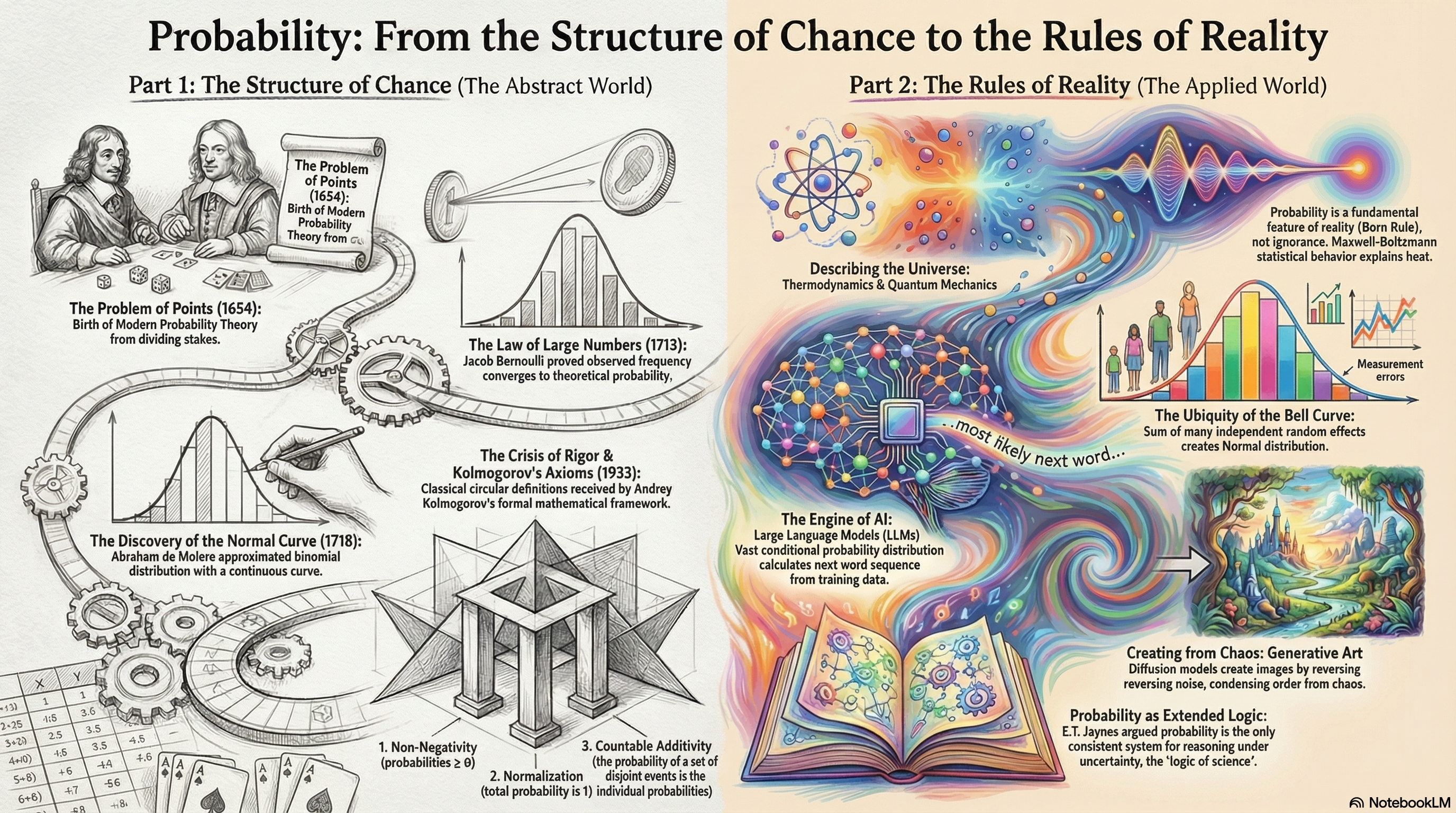
In the mid-17th century, Antoine Gombaud, the Chevalier de Méré, a French nobleman and writer, found himself perplexed by a discrepancy between his gambling intuition and his financial losses. He posed two problems to the mathematician Blaise Pascal.
The first was the “Dice Problem”: Why was betting on getting at least one ‘6’ in four rolls of a single die profitable, while betting on getting at least one ‘double-6’ in 24 rolls of two dice was not? De Méré intuitively felt the ratio of rolls (4 to 6 sides vs. 24 to 36 combinations) should preserve the probability. He was wrong, and the calculation of these odds (using the complement rule: 1 USD - (35/36)^{24}\$) revealed the non-linear nature of multiplicative probability.1
The second, and far more profound, challenge was the “Problem of Points.” This ancient puzzle asked: How should the stakes be fairly divided between two players if a game is interrupted before either has reached the required number of points to win?.2
2.3 The Correspondence of 1654: The Birth of a Discipline
During the summer of 1654, Blaise Pascal and Pierre de Fermat exchanged a series of letters that effectively invented modern probability theory. Their approach to the Problem of Points differed in method but agreed in result, establishing the dual nature of probabilistic reasoning that persists to this day: the combinatorial (counting) approach and the analytical (expectational) approach.
Fermat’s Combinatorial Method: Fermat approached the problem by imagining that the game continued for the maximum possible number of rounds needed to decide a winner. If Player A needs \$a\$ points and Player B needs \$b\$ points, the game must end within \$(a + b - 1)\$ rounds. Fermat listed every possible permutation of wins and losses over these hypothetical rounds. By counting how many of these “possible worlds” resulted in a victory for A versus B, he determined the ratio for dividing the stakes.4 This method relied on the concept of the “sample space”—the set of all possible outcomes—though the term would not be coined for centuries.
Pascal’s Method of Expectations: Pascal found Fermat’s enumeration tedious for large numbers. He developed a recursive method, now known as Backward Induction. He reasoned from the state of the game just before a win. If a player needs 0 points, the value of the game to them is the full stake (100%). If both players need equal points, the value is 50%. For any intermediate state, the value is the average of the values of the two possible subsequent states (winning the next round or losing it). For example, if the total stake is 64 pistoles, and Player A needs 1 point while Player B needs 2: If A wins the next throw, A wins 64. If A loses the next throw, the state becomes equal (both need 1 point), so A is entitled to 32. Therefore, the current value for A is the average of 64 and 32, which is 48 pistoles.4 This recursive logic introduced the concept of Mathematical Expectation (\$E[X]\$), which remains the cornerstone of modern decision theory, economics, and algorithmic reinforcement learning. Pascal later systematized these counts using his famous “Arithmetical Triangle” (Pascal’s Triangle), linking probability directly to the binomial coefficients and combinatorial mathematics.2
2.4 The Classical Era: From Games to Laws
Following the Pascal-Fermat correspondence, probability theory expanded rapidly, moving from the analysis of discrete games to continuous variables and scientific inference.
Jacob Bernoulli and the Law of Large Numbers (1713): In Ars Conjectandi, Bernoulli proved that as the number of trials in a random experiment increases, the observed frequency of an event will converge to its theoretical probability.1 This was the first bridge between the abstract “probability” (a number between 0 and 1) and physical reality (frequency of occurrence). It legitimized the use of statistics to estimate unknown probabilities from data.
Abraham de Moivre and the Normal Curve (1718): In The Doctrine of Chances, De Moivre tackled the behavior of binomial distributions for large numbers of trials. He discovered that the discrete binomial distribution could be approximated by a continuous, bell-shaped curve—the Normal Distribution.3 This was the precursor to the Central Limit Theorem and marked the entry of calculus into probability theory.
Pierre-Simon Laplace and the Scientific Method (1812): Laplace’s Théorie analytique des probabilités was a monumental synthesis. He extended probability to problems of astronomy (reducing errors in observations), jurisprudence (reliability of witnesses), and demographics. Laplace famously defined probability as the ratio of favorable cases to all possible cases, provided the cases are “equally possible”.2 This “Classical Definition” dominated the 19th century, but it contained a fatal logical flaw: it defined probability in terms of “equally possible” events—essentially defining probability by using the concept of probability.
3. The Crisis of Rigor and the Kolmogorov Synthesis
By the turn of the 20th century, mathematics faced a crisis of foundations. The paradoxes of set theory (Russell’s Paradox) and the ambiguities of the “Classical Definition” of probability made the field seem shaky compared to the rigorous new axiomatizations of geometry and algebra.
3.1 The Failure of Classical and Frequentist Definitions
The Classical definition failed when the number of outcomes was infinite (e.g., picking a random real number). The Frequentist definition (probability is the limit of relative frequency) was circular: it assumed the limit existed, which relied on the Strong Law of Large Numbers, which in turn relied on the definition of probability.
Furthermore, Bertrand’s Paradox (1889) demonstrated that for continuous problems, “equally likely” is ill-defined. If one asks for the probability that a “random chord” in a circle is longer than the side of an inscribed equilateral triangle, the answer depends entirely on the physical process of choosing the chord: Random Endpoints: Probability = 1 USD/3. USD Random Radius: Probability = 1 USD/2. USD Random Midpoint: Probability = 1 USD/4.8 USD
These contradictions proved that probability could not simply be “derived” from physical intuition; it required a rigorous, abstract mathematical structure that specified the measure explicitly before any calculation could begin.
3.2 Kolmogorov’s 1933 Axioms
The resolution came from the Russian mathematician Andrey Kolmogorov in his monograph Grundbegriffe der Wahrscheinlichkeitsrechnung (Foundations of the Theory of Probability).3 Kolmogorov’s genius was to sever probability from its interpretation (beliefs or frequencies) and treat it purely as a branch of Measure Theory, a field of real analysis developed by Borel and Lebesgue.
Kolmogorov defined a Probability Space as a triplet \$(\Omega, \mathcal{F}, P), USD where: \$\Omega\$ (Omega) is the Sample Space: The set of all possible elementary outcomes. \$\mathcal{F}\$ (Sigma-Algebra) is the Event Space: A collection of subsets of \$\Omega\$ that we are allowed to measure. \$P\$ is the Probability Measure: A function mapping events to real numbers.12
This structure resolved the paradoxes. In Bertrand’s case, specifying \$(\Omega, \mathcal{F}, P)\$ forces the mathematician to state exactly which measure they are using (e.g., uniform on radius vs. uniform on circumference), eliminating the ambiguity.
3.3 The Main Axioms of Probability
Kolmogorov condensed the entire theory into three fundamental axioms 14: Axiom 1: Non-Negativity
\$\$P(A) \ge 0 \quad \forall A \in \mathcal{F}\$\$
Reflection of Reality: In the physical world, “chance” measures the potential for existence. An event can either not occur (0) or occur (positive). “Negative probability” corresponds to no observable phenomenon in classical reality. While some quasiprobability distributions in quantum optics (like the Wigner function) can take negative values, these are not true probabilities in the Kolmogorovian sense but computational tools for phase-space analysis. The axiom anchors probability to the logic of existence.12
Axiom 2: Normalization (Unit Measure)
\$\$P(\Omega) = 1\$\$
Reflection of Reality: This is the axiom of certainty. It states that something must happen. The set of all possible outcomes \$\Omega\$ is exhaustive. If the probability of the universe of outcomes were less than 1, it would imply a “hole” in reality where no outcome occurs. If greater than 1, it implies redundant existence. This normalization allows probabilities to be compared across different contexts and scales.17
Axiom 3: Countable Additivity (\$\sigma\$-Additivity) For any countable sequence of pairwise mutually exclusive events \$E_1, E_2, \dots\$:
\$\$P\left(\bigcup_{i=1}^{\infty} E_i\right) = \sum_{i=1}^{\infty} P(E_i)\$\$
Reflection of Reality: This is the mathematical engine that allows probability to handle infinity. It implies that the probability of “at least one” of a disjoint set of events occurring is simply the sum of their individual probabilities. Finite Additivity: The sum rule for two events (\$P(A \cup B) = P(A) + P(B)\$) is intuitive. If a coin cannot be both Heads and Tails, the chance of it being “Heads or Tails” is the sum of the parts. The Infinite Extension: Countable additivity allows us to define continuous probability distributions (like the Normal distribution) where the probability of any single point is exactly 0, yet the probability of an interval is positive. Without this axiom, calculus (integration) could not be applied to probability, severing the link between probability and the laws of physics.12
4. The Philosophical Controversy: Finite vs. Infinite Universes
While Kolmogorov’s axioms are universally accepted in mathematics for their utility, Axiom 3 (Countable Additivity) remains the subject of intense debate regarding its reflection of physical reality.
4.1 The Finite Universe Objection
Skeptics argue that the physical universe appears to be finite. If space-time is discrete at the Planck scale, and the total information content of the observable universe is bounded (Bekenstein bound), then true “infinity” does not physically exist. Therefore, an axiom that dictates behavior for infinite sequences of events is a mathematical convenience, not a physical necessity.18
4.2 De Finetti and the Infinite Lottery
Bruno de Finetti, a champion of subjective Bayesianism, fiercely opposed Countable Additivity. He proposed the “Infinite Lottery”: Imagine picking a winning number from the set of all natural numbers \$\mathbb{N} = {1, 2, 3, \dots}\$ such that every number has an equal chance of being picked.
If the probability of picking any number \$n\$ is zero (\$P(n)=0\$), then by Countable Additivity, the probability of picking any number is \$\sum 0 = 0. USD This contradicts Axiom 2 (\$P(\Omega)=1\$).
If the probability is some small \$\epsilon > 0, USD then the sum diverges to infinity, also contradicting Axiom 2.
Therefore, a uniform distribution on the natural numbers is impossible under Kolmogorov’s axioms. De Finetti argued this was absurd; conceptually, we can imagine being indifferent among all integers. He argued for Finite Additivity, which permits such distributions but breaks the link with standard calculus.18
4.3 Resolution: Probability as Idealized Physics
The consensus today is that while the universe may be finite, the models we use to describe it (calculus, real numbers) are continuous and infinite. To do physics (e.g., statistical mechanics), we need integration. Countable additivity is the necessary bridge that allows us to approximate large, discrete systems (like gas molecules) as continuous fields.
It forces our probability models to “decay”—probability mass must eventually drop off (like the tails of a Bell curve) so that the sum remains 1. This matches physical observations: energy and mass are always localized, never uniformly distributed across an infinite expanse.21
5. Probability as the Logic of Science: Jaynes’ Robot
If Kolmogorov provided the syntax of probability, who defined the semantics? What does \$P(A)\$ mean?
5.1 The Logical Interpretation
E.T. Jaynes, in Probability Theory: The Logic of Science, argued that probability is neither a physical frequency nor a subjective whim. It is Extended Logic. Just as Aristotelian logic provides the rules for reasoning with certainties (If A then B), probability theory provides the unique, consistent rules for reasoning with uncertainties.22
5.2 The Reasoning Robot
Jaynes proposed a thought experiment: Design a “Reasoning Robot” to process information and form degrees of belief about propositions. We impose only simple, qualitative “desiderata” on this robot: Representation: Degrees of plausibility are represented by real numbers. Common Sense: The robot’s reasoning matches qualitative human intuition (e.g., if new evidence supports A, the plausibility of A cannot decrease). Consistency: Path Independence: If a conclusion can be reached via two different derivations, the result must be the same. Non-Ideology: The robot must use all available evidence; it cannot arbitrarily ignore information. Equivalence: Equivalent states of knowledge must yield equivalent probability assignments.23
Cox’s Theorem proves that any system satisfying these logical requirements must operate according to the rules of probability (Sum Rule and Product Rule). This was a profound result: it implies that probability is not just “one way” to handle uncertainty; it is the only consistent way. Any deviation from Bayesian probability theory inevitably leads to logical inconsistencies (Dutch Books) where the system can be tricked into contradictory beliefs.18
6. Reflections of Reality: The Normal Distribution and Thermodynamics
The abstract axioms of probability manifest in the physical world with startling ubiquity. The two most prominent examples are the Normal Distribution and the laws of Thermodynamics.
6.1 The Ubiquity of the Bell Curve
Why do human heights, measurement errors, IQ scores, and the velocities of gas particles all follow the Gaussian (Normal) distribution? It is not a coincidence; it is a mathematical inevitability driven by the Central Limit Theorem (CLT).
The CLT states that the sum (or average) of a large number of independent, identically distributed random variables will converge to a Normal distribution, regardless of the shape of the original distribution.5
Human Height: Height is determined by thousands of genetic variants and environmental factors. Each factor adds a small “plus” or “minus” to the total. The aggregate of these thousands of small, independent random effects results in a Bell curve.
Measurement Error: Any experimental measurement is subject to myriads of tiny perturbations—thermal fluctuations, atmospheric vibrations, electronic noise. The sum of these errors distributes normally.
Maximum Entropy: From an information-theoretic perspective, the Normal distribution is the distribution of “Maximum Entropy” (maximum ignorance) for a fixed mean and variance. It assumes the least amount of structure possible. Nature appears to default to this state of maximum disorder consistent with energy constraints.27
6.2 Statistical Mechanics: Deriving Physics from Probability
James Clerk Maxwell and Ludwig Boltzmann derived the fundamental laws of thermodynamics not from mechanics, but from probability.
The Derivation: Consider a gas of \$N\$ particles with total energy \$U. USD How is energy distributed among the particles? Microstates: We treat the particles as placing balls into bins (energy levels). Combinatorics: We calculate the number of ways \$W\$ to arrange particles such that the total energy is \$U. USD Maximization: We assume, based on the Principle of Indifference, that every microstate is equally likely. The macroscopic state we observe (temperature, pressure) corresponds to the configuration with the vastest number of microstates. Using Lagrange multipliers to maximize \$W\$ (or \$\ln W, USD which is Entropy), we derive the Maxwell-Boltzmann Distribution:
\$\$P(E) \propto e^{-\frac{E}{k_B T}}\$\$
Here, temperature (\$T\$) is not a fundamental quantity; it is a statistical parameter that emerges from the probability distribution of particle energies.29 This proved that the “laws” of heat are simply the laws of large numbers applied to atoms.
7. Modern Applications I: The Quantum Ontological Shift
In classical physics, probability was epistemic—it reflected our ignorance of the precise positions of particles. In Quantum Mechanics (QM), probability became ontological—it reflects the fundamental nature of reality.
7.1 The Born Rule
The connection between the abstract quantum state vector \$|\Psi\rangle\$ and physical reality is given by the Born Rule, postulated by Max Born in 1926. It states that the probability of measuring a system in a state \$|a\rangle\$ is proportional to the square of the amplitude:
\$\$P(a) = |\langle a | \Psi \rangle|^2\$\$
This rule is the linchpin of quantum theory. Without it, the Schrödinger equation is just abstract algebra. The Born Rule connects the math to the experimental clicks of a Geiger counter.32
7.2 Deriving the Rule
Is the Born Rule an axiom, or can it be derived?
Gleason’s Theorem: Mathematically, Gleason proved that in dimensions \$>2, USD the Born Rule is the only consistent probability measure on the lattice of quantum subspaces. This gives it a rigor similar to Kolmogorov’s axioms.33
Many-Worlds Interpretation (MWI): In MWI, where all outcomes occur in branching universes, deriving the Born Rule is controversial. If all outcomes happen, does “probability” make sense? Deutsch and Wallace argue that a rational agent in a branching universe would bet on outcomes according to the Born Rule to maximize utility, effectively recovering probability from decision theory.32
7.3 QBism: Quantum Bayesianism
A modern interpretation, QBism, treats the quantum state not as a description of the world, but as an observer’s belief about the world. Here, the Born Rule is an extension of the laws of consistency (Dutch Book arguments) into the quantum realm. It suggests that probability theory is the fundamental interface between the observer and the universe.25
8. Modern Applications II: Artificial Intelligence and Stochastic Computing
In the 21st century, probability has become the engine of Artificial Intelligence. The generative AI revolution—from ChatGPT to Stable Diffusion—is essentially an industrial-scale application of advanced probability theory.
8.1 Large Language Models (LLMs) as Probability Engines
At its core, an LLM is a conditional probability distribution estimating the likelihood of the next word (token) given a sequence of previous words:
\$\$P(w_t | w_{t-1}, w_{t-2}, \dots, w_1)\$\$
The model does not “know” facts; it knows the probability of token co-occurrences in the training data.
Sampling and Temperature: The model produces a vector of “logits” (raw scores) for every possible word. These are converted to probabilities using the Softmax function with a Temperature parameter (\$T\$):
\$\$P_i = \frac{\exp(z_i / T)}{\sum \exp(z_j / T)}\$\$ High Temperature (\$T > 1\$): The distribution flattens (Entropy increases). The model becomes more random, “creative,” and prone to hallucination. Low Temperature (\$T < 1\$): The distribution sharpens (Entropy decreases). The model becomes deterministic and repetitive.35
Nucleus Sampling (Top-p): To prevent the model from choosing absurdly low-probability words, methods like Top-p sampling are used. The model sums the probabilities of the most likely words until the sum reaches a threshold \$p\$ (e.g., 0.95), and samples only from that “Nucleus.” This dynamically adjusts the vocabulary size based on the model’s confidence—a direct application of Kolmogorov’s Axiom 2 (Normalization) to control algorithmic output.37
8.2 Generative Art: Diffusion Models and Langevin Dynamics
Text-to-Image models (like Stable Diffusion) utilize Diffusion Probabilistic Models. These models are trained to reverse the process of entropy. Forward Process: A Markov chain gradually adds Gaussian noise to an image until it becomes pure random static. This simulates a physical diffusion process (like ink spreading in water). Reverse Process: The AI learns to reverse time, predicting the original image from the noise.
Langevin Dynamics: Mathematically, this generation process is modeled using Stochastic Differential Equations (SDEs) and Langevin Dynamics. The process moves the image along the gradient of the data distribution (moving towards “likely” images) while adding a specific amount of noise to avoid getting stuck in local optima.
\$\$x_{t+1} = x_t + \frac{\epsilon}{2} \nabla_x \log p(x) + \sqrt{\epsilon} z_t\$\$
This equation connects modern AI generation directly to the physics of Brownian motion modeled by Paul Langevin in 1908. The AI is literally “condensing” order out of chaos using the laws of statistical mechanics.39
8.3 Stochastic Gradient Descent (SGD)
The training of these massive neural networks relies on Stochastic Gradient Descent. Computing the true gradient of the loss function over terabytes of data is impossible. Instead, we estimate the gradient using small, random batches of data.
Why it works: The expected value of the stochastic gradient is the true gradient. Furthermore, the “noise” introduced by the random sampling helps the optimization algorithm escape saddle points in the high-dimensional loss landscape, acting as a form of regularization. The randomness is not a bug; it is a feature that allows learning to generalize.42
9. The Metaphysics of Probability: Knowledge, Information, and Infinite Divisibility
Recent interdisciplinary synthesis has illuminated a profound connection between the mathematical structure of probability and ancient metaphysical concepts of “The One” and “The Many.” By refining the definitions of “Information” and “Knowledge” through the lens of modern probability, we can mathematically formalize how a unified reality decentralizes into infinite diversity while retaining its singularity.
9.1 Formalizing the Distinction: Signal vs. Noise
To understand this mechanism, we must first rigorously define our terms using Information Theory and Kolmogorov’s framework: Information (\$\mathcal{I}\$) is the Realization of a stochastic process. It corresponds to Vikara (modification/change). It is the specific, historical path taken by reality—the “noise.” In a coin flip experiment, getting a sequence of “H, T, T, H…” is information. It is high-entropy, expensive to store, and “lossy” because a single realization does not fully capture the underlying law.
Knowledge (\$\mathcal{K}\$) is the Probability Measure itself. It corresponds to Atman (the invariant self). It is the “signal”—the compressed, invariant algorithm (\$P(H)=0.5\$) that generates the information. Knowledge is “lossless” because it describes the potential of all possible paths.
9.2 The Mechanism of Decentralization: Infinite Divisibility
How does the “One” (Knowledge) become the “Many” (Information) without losing its nature? The mathematical answer lies in the concept of Infinite Divisibility.
A probability distribution \$F\$ is defined as Infinitely Divisible if, for any integer \$n, USD it can be represented as the sum of \$n\$ independent, identically distributed (i.i.d.) random variables:
\$\$Y = X_1 + X_2 + \dots + X_n\$\$
This concept mirrors the metaphysical process of Decentralization. The Whole in the Parts: The properties of the macroscopic “Whole” (\$Y\$) are encoded in the microscopic “Parts” (\$X_i\$). For example, the Normal distribution is infinitely divisible; if you slice a Bell Curve into \$n\$ parts, the parts are also Bell Curves (with scaled variance).
Lévy Stability: This decentralization is governed by Lévy Stability, which ensures that the sum of independent copies of a variable retains the same distribution shape as the original. This is the mathematical proof that “Atman reflects as a full copy.” Whether we look at the height of one oak tree (a realization/Information) or the distribution of a forest (the law/Knowledge), the underlying “code” is invariant.
9.3 The Unity of the Whole: Normalization as Atman
The most striking feature of this framework is how it resolves the “One vs. Many” paradox through Kolmogorov’s Normalization Axiom:
\$\$P(\Omega) = 1\$\$
No matter how infinitely divisible the system is, and no matter how many trillions of independent “form factors” (realizations/Vikara) are generated, the total probability mass must always sum to exactly One.
Conservation of Existence: Just as energy is conserved, “possibility” is conserved. The infinite diversity of the manifest world (Information) is merely a decentralized expression of a singular, unified Probability Measure (Knowledge).
The Grand Scheme: In this view, the “Normal Distribution” observed in nature is not just a statistical artifact; it is the visible signature of the “One” (Knowledge) dispersing itself into the “Many” (Information) through the mechanism of infinite divisibility, while strictly adhering to the unity of the Normalization axiom.
10. The Pedagogical Imperative: Probability vs. The Calculus Hegemony
Despite its centrality to modern science and technology, probability theory is often marginalized in high school curricula in favor of Calculus. This “Calculus Trap” is increasingly challenged by educators and statisticians who argue that probabilistic literacy is a prerequisite for modern citizenship.
10.1 The Case for Statistics Over Calculus
Mathematician Arthur Benjamin argues that the “summit” of high school math should be statistics, not calculus.
Utility: Calculus is essential for engineers and physicists. Probability is essential for everyone. Doctors must interpret test sensitivities; voters must interpret polls; investors must interpret risk.
The Data Age: We live in a world of Big Data. Understanding distributions, variability, and correlation is arguably more critical for the average citizen than computing the volume of a solid of revolution.44
10.2 Cognitive Biases and the GAISE Report
Research by Daniel Kahneman and Amos Tversky exposed the fragility of human intuition regarding chance. We suffer from systematic “Cognitive Biases”: Base Rate Neglect: Ignoring general prevalence information (e.g., assuming a medical test is accurate without considering how rare the disease is). Conjunction Fallacy: Believing specific conditions are more probable than general ones (e.g., thinking “Linda is a feminist bank teller” is more likely than “Linda is a bank teller”).46
The GAISE (Guidelines for Assessment and Instruction in Statistics Education) reports emphasize that education must focus on “Statistical Literacy”—the ability to reason with data and uncertainty—rather than just procedural calculation. By formally teaching probability, we equip students with the cognitive tools to overcome these innate biases, making them less susceptible to manipulation by misleading statistics in media and politics.48
11. Disciplinary Identity: Mathematics or Science?
Finally, we address the standing of the field itself. Should Probability be its own subject, distinct from Pure Mathematics?
11.1 The Argument for Separation
Probability and Statistics possess a distinct epistemology from Pure Math.
Inductive vs. Deductive: Pure Math is deductive (Axioms \$\to\$ Theorems). Statistics is often inductive (Data \$\to\$ Inference).
Falsifiability: Statistical models are scientific hypotheses about the world, subject to empirical validation. A mathematical proof is eternally true; a statistical model is only “useful” or “not useful”.51
The Science of Data: Many argue that Statistics is a separate science (Data Science) that uses mathematics, much like Physics uses mathematics, but is defined by its own focus on uncertainty and measurement.52
11.2 The Argument for Unity
However, the foundations of probability are firmly rooted in Pure Analysis.
Measure Theory: As Kolmogorov showed, probability is a subset of Measure Theory. To understand advanced concepts like Brownian Motion, Stochastic Calculus (Itô Calculus), or the convergence of random variables, one requires the rigorous machinery of Real Analysis and Topology.
Interconnectedness: Probability has deep connections to Number Theory (Riemann Hypothesis and Random Matrices), Geometry, and Logic. Severing it from math would impoverish both fields.
Synthesis: Probability occupies a unique “Superposition.” Its axiomatic core is pure mathematics. Its interpretive logic (Bayesianism) is philosophy. Its application (Statistics, AI, Physics) is empirical science. It is the bridge between the abstract world of logic and the noisy world of data.
12. Conclusion
Who postulated probability theory? It was not a single mind, but a centuries-long dialogue between the specific and the general. It began with Cardano and De Méré observing the idiosyncrasies of dice. It was birthed as a mathematical discipline by Pascal and Fermat in the summer of 1654. It was expanded into a description of the natural world by Bernoulli, De Moivre, and Laplace. And finally, it was crystallized into a rigorous axiomatic structure by Andrey Kolmogorov in 1933.
The axioms of Non-Negativity, Normalization, and Countable Additivity are not merely dry mathematical rules. They are the structural pillars of rational thought. They reflect a universe that is consistent, unitary, and continuous.
From the thermodynamic distribution of stars to the generative algorithms of artificial intelligence, probability theory remains the most effective tool humanity has devised to navigate the unknown. It is, as Jaynes argued, the logic of science itself—the rigorous calculus of common sense in a world of uncertainty. Data Tables and Comparisons Table 1: The Evolution of Probability Definitions
| Era | Definition of Probability | Proponent | Key Limitation |
|---|---|---|---|
| Pre-1650 | Qualitative / Propensity | Aristotle, Cardano | Lack of mathematical quantification; reliance on “fate.” |
| 1654-1800 | Classical Ratio | Pascal, Laplace | Defined as ratio of “Equally Likely” outcomes. Circular definition; fails for infinite sets (Bertrand’s Paradox). |
| 1800-1930 | Frequentist Limit | Venn, Von Mises | Limit of relative frequency as \$N \to \infty. USD Circular reliance on LLN; cannot handle unique events. |
| 1933-Present | Axiomatic Measure | Kolmogorov | defined on \$(\Omega, \mathcal{F}, P). USD Mathematically rigorous; interpretation-agnostic. |
| 1950-Present | Subjective Bayesian | De Finetti, Savage, Jaynes | Degree of belief / Logical plausibility. Requires priors; debate over objectivity. |
Table 2: Probability Sampling in AI (LLMs)
| Parameter | Mechanism | Effect on Output | Use Case |
|---|---|---|---|
| Temperature (\$T\$) | Scales logits before Softmax: \$P_i \propto e^{z_i/T}\$ | High T: Increases diversity, randomness. | High for creative writing; Low for coding/logic. |
| Low T: Increases determinism, repetition. | |||
| Top-k | Samples from top \$k\$ tokens only. | Prevents wild hallucinations by cutting off the “long tail” of low-probability words. | General purpose generation. |
| Nucleus (Top-p) | Samples from smallest set summing to \$p. USD | Dynamic vocabulary size. Balances diversity and coherence better than Top-k. | Modern standard for high-quality text generation. |
References
- History of Probability | Research Starters - EBSCO, accessed December 9, 2025, https://www.ebsco.com/research-starters/mathematics/history-probability
- History of probability - Wikipedia, accessed December 9, 2025, https://en.wikipedia.org/wiki/History_of_probability
- Birth of probability theory - SCIENCE, accessed December 9, 2025, https://jfgouyet.fr/en/birth-of-probability-theory/
- FERMAT AND PASCAL ON PROBABILITY - University of York, accessed December 9, 2025, https://www.york.ac.uk/depts/maths/histstat/pascal.pdf
- Chapter 7 Central Limit Theorem and law of large numbers | Foundations of Statistics, accessed December 9, 2025, https://bookdown.org/peter_neal/math4081-lectures/Sec_CLT.html
- Probability theory - Central Limit, Statistics, Mathematics | Britannica, accessed December 9, 2025, https://www.britannica.com/science/probability-theory/The-central-limit-theorem
- The Unifying Framework of Probability: Interpretations and Axioms | by Gadeabhishekreddy | Nov, 2025 | Medium, accessed December 9, 2025, https://medium.com/@gadeabhishekreddy/the-unifying-framework-of-probability-interpretations-and-axioms-7abd697f3134
- Bertrand’s Paradox Resolution and Its Implications for the Bing–Fisher Problem - MDPI, accessed December 9, 2025, https://www.mdpi.com/2227-7390/11/15/3282
- Bertrand’s Paradox and the Principle of Indifference | Philosophy of …, accessed December 9, 2025, https://www.cambridge.org/core/journals/philosophy-of-science/article/bertrands-paradox-and-the-principle-of-indifference/DC735A7B90AD19EB0572A5EA9C5B07BB
- Andrei Nikolaevich Kolmogorov (1903-1987) - Utah State University, accessed December 9, 2025, https://www.usu.edu/math/schneit/StatsHistory/Probabilists/Kolmogorov
- Foundations of Probability Theory - Assets - Cambridge University Press, accessed December 9, 2025, https://assets.cambridge.org/97811084/18744/excerpt/9781108418744_excerpt.pdf
- Probability axioms - Wikipedia, accessed December 9, 2025, https://en.wikipedia.org/wiki/Probability_axioms
- Kolmogorov and Probability Theory - CORE, accessed December 9, 2025, https://core.ac.uk/download/pdf/268083255.pdf
- Kolmogorov Axioms - acemate | The AI, accessed December 9, 2025, https://acemate.ai/glossary/kolmogorov-axioms
- Probability axioms | Thinking Like a Mathematician Class Notes - Fiveable, accessed December 9, 2025, https://fiveable.me/thinking-like-a-mathematician/unit-6/probability-axioms/study-guide/tW61rdJMoeWxXQgU
- Understanding Probability and Its Fundamental Axioms - sunrise classes, accessed December 9, 2025, https://www.sunriseclassesiss.com/post/understanding-probability-and-its-fundamental-axioms
- Axiomatic Definition of Probability Explained with Examples - Vedantu, accessed December 9, 2025, https://www.vedantu.com/maths/axiomatic-definition-of-probability
- Why Countable Additivity? - Joel Velasco, accessed December 9, 2025, https://joelvelasco.net/teaching/5311/easwaran14-whyCountable.pdf
- A debate about the physics of the universe and the concept of infinity. : r/AskPhysics - Reddit, accessed December 9, 2025, https://www.reddit.com/r/AskPhysics/comments/1gez0tw/a_debate_about_the_physics_of_the_universe_and/
- LOST CAUSES IN STATISTICS I: Finite Additivity | Normal Deviate - WordPress.com, accessed December 9, 2025, https://normaldeviate.wordpress.com/2013/06/30/lost-causes-in-statistics-i-finite-additivity/
- Against countable additivity - Wolfgang Schwarz, accessed December 9, 2025, https://www.umsu.de/blog/2013/598
- Probability Theory: The Logic of Science - Department of Mathematics and Statistics, accessed December 9, 2025, http://www.mscs.dal.ca/~gabor/book/cpreambl.ps.gz
- Book Notes: Probability Theory by E.T. Jaynes — Ad Astra Major, accessed December 9, 2025, https://www.adastramajor.com/aam-blog/2019/5/24/book-notes-probability-theory-by-et-jaynes
- The reasoning robot, Jaynes’ desiderata, and Cox’s Theorem | Scrub Physics, accessed December 9, 2025, https://leepavelich.wordpress.com/2014/08/26/the-reasoning-robot-jaynes-desiderata-and-coxs-theorem/
- [2012.14397] Born’s rule as a quantum extension of Bayesian coherence - arXiv, accessed December 9, 2025, https://arxiv.org/abs/2012.14397
- Central limit theorem: the cornerstone of modern statistics - PMC, accessed December 9, 2025, https://pmc.ncbi.nlm.nih.gov/articles/PMC5370305/
- Why is the normal distribution considered a universal phenomenon? - Reddit, accessed December 9, 2025, https://www.reddit.com/r/AskScienceDiscussion/comments/ajoq9g/why_is_the_normal_distribution_considered_a/
- Why is normal distribution so ubiquitous? - Let’s talk about science!, accessed December 9, 2025, https://ekamperi.github.io/mathematics/2021/01/29/why-is-normal-distribution-so-ubiquitous.html
- The Boltzmann factor: A simplified derivation - Technische Universität Braunschweig, accessed December 9, 2025, https://www.tu-braunschweig.de/index.php?eID=dumpFile&t=f&f=138377&token=ce78f1a73be3528669c0a5a4a6675d0e3284b02e
- Maxwell–Boltzmann distribution - Wikipedia, accessed December 9, 2025, https://en.wikipedia.org/wiki/Maxwell%E2%80%93Boltzmann_distribution
- Maxwell Boltzmann Distribution Derivation - BYJU’S, accessed December 9, 2025, https://byjus.com/physics/maxwell-boltzmann-distribution-derivation/
- Born rule - Wikipedia, accessed December 9, 2025, https://en.wikipedia.org/wiki/Born_rule
- Derivations of the Born Rule - PhilSci-Archive, accessed December 9, 2025, https://philsci-archive.pitt.edu/15943/1/BornRule24-4-19.pdf
- Bayes’ rule goes quantum - Physics World, accessed December 9, 2025, https://physicsworld.com/a/bayes-rule-goes-quantum/
- What is LLM Temperature? - IBM, accessed December 9, 2025, https://www.ibm.com/think/topics/llm-temperature
- LLM Parameters Explained: A Practical, Research-Oriented Guide with Examples, accessed December 9, 2025, https://promptrevolution.poltextlab.com/llm-parameters-explained-a-practical-research-oriented-guide-with-examples/
- Understanding Temperature, Top-k, and Top-p Sampling in Generative Models - Codefinity, accessed December 9, 2025, https://codefinity.com/blog/Understanding-Temperature%2C-Top-k%2C-and-Top-p-Sampling-in-Generative-Models
- Top-p sampling - Wikipedia, accessed December 9, 2025, https://en.wikipedia.org/wiki/Top-p_sampling
- What are Diffusion Models? | Lil’Log, accessed December 9, 2025, https://lilianweng.github.io/posts/2021-07-11-diffusion-models/
- Lecture 3 – Langevin algorithms 3.1 Introduction - metaphor, accessed December 9, 2025, https://metaphor.ethz.ch/x/2024/fs/401-4634-DRL/lec/Lecture03.pdf
- (PDF) Diffusion models learn distributions generated by complex Langevin dynamics, accessed December 9, 2025, https://www.researchgate.net/publication/386419325_Diffusion_models_learn_distributions_generated_by_complex_Langevin_dynamics
- Stochastic gradient descent - Wikipedia, accessed December 9, 2025, https://en.wikipedia.org/wiki/Stochastic_gradient_descent
- Stochastic Gradient Descent in Theory and Practice - Stanford AI Lab, accessed December 9, 2025, https://ai.stanford.edu/~optas/data/stanford_qual_exams.pdf
- Math that Matters: The Case for Probability over Polynomials - Anand Sanwal, accessed December 9, 2025, https://anandsanwal.me/math-eduction-more-probability-statistics-less-calculus/
- Arthur Benjamin: Teach statistics before calculus! - Andrew B. Collier / @datawookie, accessed December 9, 2025, https://datawookie.dev/blog/2016/07/arthur-benjamin-teach-statistics-before-calculus/
- Gerd Gigerenzer on the legacy of Daniel Kahneman, accessed December 9, 2025, https://statmodeling.stat.columbia.edu/2025/12/03/gerd-gigerenzer-on-the-legacy-of-daniel-kahneman/
- kahneman-tversky.pdf, accessed December 9, 2025, https://home.cs.colorado.edu/~martin/Csci6402/Papers/kahneman-tversky.pdf
- Guidelines for Assessment and Instruction in Statistics Education - Wikipedia, accessed December 9, 2025, https://en.wikipedia.org/wiki/Guidelines_for_Assessment_and_Instruction_in_Statistics_Education
- Guidelines for Assessment and Instruction in Statistics Education (GAISE) - Stat@Duke, accessed December 9, 2025, https://www2.stat.duke.edu/courses/Fall12/sta790.04/GAISE.pdf
- Guidelines for Assessment and Instruction in Statistics Education (GAISE) in Statistics Education (GAISE) College Report College - Montgomery College, accessed December 9, 2025, https://www.montgomerycollege.edu/_documents/offices/elite/gaise-college.pdf
- Why are mathematics and statistics considered two different subjects in college? - Quora, accessed December 9, 2025, https://www.quora.com/Why-are-mathematics-and-statistics-considered-two-different-subjects-in-college
- Why is statistics considered a different discipline than mathematics rather than as a branch of mathematics?, accessed December 9, 2025, https://math.stackexchange.com/questions/1970337/why-is-statistics-considered-a-different-discipline-than-mathematics-rather-than
Tips and Donations
If you enjoyed this deep dive, consider supporting the project with a tip in Sats. It’s a simple, global way to support independent research.
To send Sats, you’ll need a lightning wallet.